Image Programming in JavaScript: The Histogram
Recently, I've spent a lot of my time taking photographs. When I get home from taking pictures, I immediately pop open Lightroom to import the images, pick out my favorites, do some adjustments on them, and publish them.
As a programmer, though, it was bothering me that I don't know exactly what's happening behind the scenes when I adjusted my images. What's really happening when I adjust the "saturation" slider for a photo? How does sharpening work, and what does its "amount" mean?
Sure, I could go read books to find out, but there's only way to really know what's happening: write a program to do it. This article represents part 1 of what will hopefully become a series on programming the digital image with JavaScript.
Wait, JavaScript?
Sure thing! With the recent adoption of the <canvas> element into modern browsers, JavaScript has gained the ability to load, display, and manipulate images at the pixel level. In addition, Jacob Seidelin recently created the Pixastic library to do the heavy DOM and canvas lifting for us.
As much as possible, I'll be using Pixastic as a base because JavaScript is a reasonably enjoyable programming language, the framework is new and simple, and I can show neat demos right in the browser. I'll also be using jQuery, because it makes writing cross-browser JavaScript much more pleasant.
Jumping Right In: What Is a Digital Image?
In the spirit of YAGNI, we're going to accept a superficial answer to this question, at least for now. We're basically going to pretend that all images are in color and represented in the same color space in the same way. Our provisional definition of a digital image is this:
A Digital Image is a sequence of pixels, each of which is represented by a 3-byte tuple (red, green, blue). The value of each element represents the strength of that color in that pixel.
This means that each pixel has a value between 0 and 255, where 0 represents absence and 255 full strength. For example, the tuple (255, 0, 0) would represent a pure red pixel, the tuple (0, 255, 0) a pure green one, and (0, 0, 255) a pure blue one.
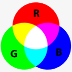
Since we're mixing light1, the colors are additive, which means that they get lighter when mixed. Thus (255, 255, 0) represents a mixture of red and green which produces yellow, (0, 255, 255) represents green and blue combined to form magenta, and so on as you can see in the chart to the right.
You can think of it is as if you're in a dark room shining colored flashlights on a wall; if you don't shine any lights the wall remains black. If you shine all three colors on it, you get white. Thus, it makes sense that (0, 0, 0) represents black and (255, 255, 255) represents white.
OK, I get it. So what's a Histogram?
There are of course lots of colors in between the pure ones I talked about above, represented by the all the possible color tuples with values between 0 and 255. In order to understand an image at a glance, it's often helpful to see just how often each color occurs in that image. The histogram allows us to do just that.
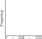
To the right is the basic schematic of a histogram. The y-axis represents the frequency of each color value, which are represented on the x-axis. The left side of the histogram shows darker colors and the right side lighter.
The histogram of an image is a chart of how often each possible value or range of values for a color occurs in that image
Below is an image next to the histograms for its red, green, and blue values, respectively.
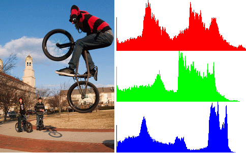
We can see that there are a lot of light blues, presumably in the the sky, a lot of midrange reds and greens, and not a whole lot of dark colors, though there is a spike at pure black. I won't go over what a histogram means for your photography; you should read what a better photographer has to say about that.
On To The Source
There are 2 major steps in creating histograms: gathering the data and drawing the histogram. To gather the data, we'll initialize three arrays with 256 slots, one array slot for each of the color values. Then we'll just loop through each pixel in the image and add one in the appropriate histogram slot for each color. That's it!
function array256(default_value) {
  arr = [];
  for (var i=0; i<256; i++) { arr[i] = default_value; }
  return arr;
}

var rvals = array256(0);
var gvals = array256(0);
var bvals = array256(0);

each_pixel(image_data, function(r, g, b) {
  rvals[r]++;
  gvals[g]++;
  bvals[b]++;
});
Where each_pixel is simply a function that loops through the image and passes the red, green, and blue value of each pixel of its first argument to the function passed as its second argument. What we have at the end of this code is three arrays, each containing the count of each possible value of one color in the image.
To simplify the display of these histograms, we'll draw on a <canvas> 256 pixels wide, so that each possible color occupies one pixel. Since our canvas is only 100 pixels tall, and any histogram value could be greater than 100, we'll scale each value as the percentage of the maximum value in the histogram.
//get a reference to the canvas to draw on
var ctx = $("#colorhistcanvas")[0].getContext("2d");
var rmax = Math.max.apply(null, rvals);
var bmax = Math.max.apply(null, bvals);
var gmax = Math.max.apply(null, gvals);

function colorbars(max, vals, color, y) {
  ctx.fillStyle = color;
  jQuery.each(vals, function(i,x) {
    var pct = (vals[i] / max) * 100;
    ctx.fillRect(i, y, 1, -Math.round(pct));
  });
}

colorbars(rmax, rvals, "rgb(255,0,0)", 100);
colorbars(gmax, gvals, "rgb(0,255,0)", 200);
colorbars(bmax, bvals, "rgb(0,0,255)", 300);
You can see this code in action at the top half of the histogram demo page. Note that the histograms on that page are being generated by JavaScript when you load the page, so you can look into the source and see exactly how the process works.
A Mean Feat
Most of the time, the three histograms are more information than we need. Instead, we want to be able to tell at a glance whether we've overexposed or underexposed the shot, and a single histogram can give us all the information we need. In this case, all we need is an average of the three histograms.
The obvious way to average the three histograms is to weight them all equally, sum each value, and divide by three. You'll see this histogram under "Average" on the demo page.
However, not all colors appear equally bright to human eyes, so the equally weighted histogram is commonly replaced with one more heavily weighted towards green, which appears brightest. A commonly given figure is 30% red, 59% green, and 11% blue, the results of which you can see in the "weighted average" histogram on the demo.
Conclusion
Hopefully, this article lays a solid base on which I can begin building up to show more complex and interesting image transformations with JavaScript and Pixastic. It should have given you a basic understanding of how an image is formed and how to build several different types of histograms from it. For a more detailed understanding, I encourage you to study the code given in the demo page; it should all be pretty simple.
If you have any questions or comments, please feel free to drop me an email.