Drawing Presentable Trees
by Bill Mill
When I needed to draw some trees for a project I was doing, I assumed that there would be a classic, easy algorithm for drawing neat trees. What I found instead was much more interesting: not only is tree layout an NP-complete problem1, but there is a long and interesting history behind tree-drawing algorithms. I will use the history of tree drawing algorithms to introduce central concepts one at a time, using each of them to build up to a complete O(n) algorithm for drawing attractive diagrams of trees.
What's the problem here?
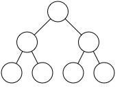
figure 1
In order to store the results of the tree drawing algorithms, we'll create a DrawTree data structure to mirror the tree we're drawing; the only thing we'll assume is that each tree node can iterate over its children. A basic implementation of DrawTree can be found in Listing 1.
class DrawTree(object):
    def __init__(self, tree, depth=0):
        self.x = -1
        self.y = depth
        self.tree = tree
        self.children = [DrawTree(t, depth+1) for t in tree]
As the sophistication of our methods increase, so will the complexity of DrawTree. For now, it just assigns -1 to the x coordinate of each node, the depth of the node to its y coordinate, and stores a reference to the root of the current tree. Then it builds up a list of the children of that node by recursively creating a DrawTree for each one. In this way, we build a DrawTree that wraps the tree it's going to draw and adds drawing-specific information to each node.
As we go along implementing better algorithms throughout this article, we'll use our experience with each to help us generate principles that will aid us in constructing the next one. Although generating an "attractive" tree diagram is matter of taste, these principles will help to guide us in improving the output of our programs.
In the beginning, there was Knuth
The particular type of drawing that we'll be making is one where the root is at the top, its children are below it, and so on. This type of diagram, and thus this entire class of problems, owes largely to Donald Knuth2, from whom we will draw our first two principles:
Principle 1: The edges of the tree should not cross each other.
Principle 2: All nodes at the same depth should be drawn on the same horizontal line. This helps make clear the structure of the tree.
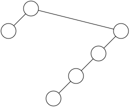
figure 2
The Knuth algorithm has the advantage of simplicity and blazing speed, but it only works on binary trees and it can produce some fairly misshapen drawings. It is a simple inorder traversal of a tree, with a global counter that is used as the x variable, then incremented at each node. The code in Listing 2 demonstrates this technique.
i = 0
def knuth_layout(tree, depth):
    if tree.left_child:
        knuth_layout(tree.left_child, depth+1)
    tree.x = i
    tree.y = depth
    i += 1
    if tree.right_child:
        knuth_layout(tree.right_child, depth+1)
As you can see from Figure 2, this algorithm produces a tree that satisfies Principle 1, but is not particularly attractive. You can also see that Knuth diagrams will grow wide very quickly, since they will not reuse x coordinates even when the tree could be significantly narrower. To avoid this waste of space, we'll introduce a third principle:
Principle 3: Trees should be drawn as narrowly as possible.
A Brief Refresher
Before we go on towards some more advanced algorithms, It's probably a good idea to stop and agree on the terms we'll use in this article. First, we're going to make use of a metaphor to family trees when describing the relationships between our data nodes. A node can have children below it, siblings to its left or right, and a parent above it.
We already talked about inorder tree traversals, and we're also going to talk about preorder and postorder traversals.. You probably saw these three terms on a "Data Structures" test a long time ago, but unless you've been playing with trees lately, they may have gotten a bit hazy.
The traversal types simply determine when we do the processing we need to do on a given node. Inorder traversal, as in the Knuth algorithm above, only applies to binary trees, and means that we process the left child, then process the current node, then finally the right child. Preorder traversal means we process the current node, then all its children, and posterder traversal is simply the reverse.
Finally, you may have seen the concept of Big O notation before as a way to express the order of magnitude of the run time for an algorithm. In this article, we're going to play fast and loose with it, using it as a simple tool to distinguish acceptable runtimes from unacceptable ones. If an algorithm already in its main loop frequently loops through all the children of one of its nodes, we're going to call it O(n^2), or quadratic. Anything else we're going to call O(n), or linear. If you want more details, the papers referenced at the end of this article contain a great deal more about the runtime characteristics of these algorithms.
From the Bottom Up
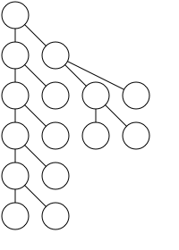
figure 3
nexts = [0] * maximum_depth_of_tree

def minimum_ws(tree, depth=0):
    tree.x = nexts[depth]
    tree.y = depth
    nexts[depth] += 1
    for c in tree.children:
        minimum_ws(c, depth+1)
Although it satisfies all of our principles, perhaps you will agree that the output is ugly. Even on a simple example such as that in Figure 3, it's difficult to quickly ascertain the relationships between the nodes, and the whole thing seems smooshed together. It's about time we introduce another principle that would help clean up both the Knuth tree and the minimum width tree:
Principle 4: A parent should be centered over its children.
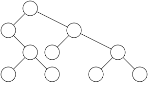
figure 4
Up to now, we've been able to get away with very simple algorithms to draw trees because we've not really had to consider local context; we've relied on global counters to keep our nodes from overlapping each other. In order to satisfy the principle that a parent should be centered over its children, we'll need to consider each node's local context, and so a few new strategies are necessary.
The first strategy that Wetherell and Shannon introduce is to build trees up from the bottom with a post-order traversal of the tree, instead of going from the top down like Listing 2, or through the middle like Listing 3. Once you look at the tree this way, centering the parent is an easy operation - simply divide its children's x coordinates in half.
We must remember, though, to stay mindful of the left side of the tree when constructing the right. Figure 4 shows a scenario where the right side of the tree has been pushed out to the right in order to accommodate the left. To accomplish this separation, Wetherell and Shannon maintain the array of next available spots introduced with Listing 2, but only use the next available spot if centering the parent would cause the right side of the tree to overlap the left side.
The Mods and the Rockers
Before we start looking at more code, let's take a closer look at the consequences of our bottom up construction of the tree. We'll give each node the next available x coordinate if it's a leaf, and center it above its children if it's a branch. However, if centering the branch will cause it to come into conflict with another part of the tree, we need to move it to the right far enough to avoid the conflict.
When we move a branch to the right, we have to move all of its children, or else we will have lost the centered parent node that we've been working so hard to maintain. It's easy to come up with a naive function to move a branch and its subtrees to the right by some number:
def move_right(branch, n):
    branch.x += n
    for c in branch.children:
        move_right(c, n)
It works, but presents a problem. If we use this function to move a subtree to the right, we'll be doing recursion (to move the tree) inside of recursion (to place the nodes), which means we'll have an inefficient algorithm which may run in time O(n^2).
To solve this problem, we'll give each node an additional member called mod. When we come to a branch that we need to move to the right by n spaces, we'll add n to its x coordinate and to its mod value, and happily continue along with the placement algorithm. Because we're moving from the bottom up, we don't need to worry about the bottom of our trees coming into conflict (we've already shown they're not), and we'll wait until later to move them to the right.
Once the first tree traversal has taken place, we run a second tree traversal to move the branches to the right that need to be moved to the right. Since we'll visit each node once and perform only arithmetic on it, we can be sure that this traversal will be O(n) just like the first one is, and together that they will be O(n) as well.
The code in Listing 5 demonstrates both the centering of parent nodes and the use of mod values to improve the efficiency of our code.
from collections import defaultdict

class DrawTree(object):
    def __init__(self, tree, depth=0):
        self.x = -1
        self.y = depth
        self.tree = tree
        self.children = [DrawTree(t, depth+1) for t in tree]
        self.mod = 0

def layout(tree):
    setup(tree)
    addmods(tree)
    return tree

def setup(tree, depth=0, nexts=None, offset=None):
    if nexts is None:  nexts  = defaultdict(lambda: 0)
    if offset is None: offset = defaultdict(lambda: 0)

    for c in tree.children:
        setup(c, depth+1, nexts, offset)

    tree.y = depth

    if not len(tree.children):
        place = nexts[depth]
        tree.x = place
    elif len(tree.children) == 1:
        place = tree.children[0].x - 1
    else:
        s = (tree.children[0].x + tree.children[1].x)
        place = s / 2

    offset[depth] = max(offset[depth], nexts[depth]-place)

    if len(tree.children):
        tree.x = place + offset[depth]

    nexts[depth] += 2
    tree.mod = offset[depth]

def addmods(tree, modsum=0):
    tree.x = tree.x + modsum
    modsum += tree.offset

    for t in tree.children:
        addmods(t, modsum)
Trees as Blocks
While it does produce good results in many cases, Listing 5 can produce some disfigured trees, such as the one in Figure 5 (ed: sadly, lost to the sands of time). A further difficulty in interpreting the trees produced by the Wetherell-Shannon algorithm is that the same tree structure, when placed at a different point in the tree, may be drawn differently. To avoid this, we'll steal a principle from a paper by Edward Reingold and John Tilford4:
Principle 5: A subtree should be drawn the same no matter where in the tree it lies.
Even though this may widen our drawings a bit, this principle will help to make them convey more information. It will also help to simplify our bottom-up traversal of the tree, since one of its consequences is that once we've figured out the x coordinates of a subtree, we only need to move it left or right as a unit.
Here is a sketch of the algorithm implemented in Listing 6:
• Do a post-order traversal of the tree
• if the node is a leaf, give it an x coordinate of 0
• else, place its right subtree as close to the left as possible without conflict
    • Use the same mod technique as in the previous algorithm to move the tree in O(n) time
• place the node halfway between its children
• Do a second walk of the tree, adding the
  accumulated mod value to the x coordinate
This algorithm is simple to the point of brilliance, but to execute it we'll need to introduce a bit of complexity.
Contours
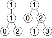
figure 6
To find the left contour of the right tree, we again take the x-coordinate of the leftmost node on each level, giving us [1,0,1]. This time, the contour has an interesting property that not all nodes are connected in a parent-child relationship; the 0 on the second level is not the parent of the 1 on the third.
If we were to join these two trees according to Listing 6, we could find the right contour of the left tree, and the left contour of the right tree. Then we could easily find the smallest amount that we needed to push the right tree to the right so that it didn't overlap the left tree. A simple method for doing so is given in Listing 7.
from operator import lt, gt

def push_right(left, right):
    wl = contour(left, lt)
    wr = contour(right, gt)
    return max(x-y for x,y in zip(wl, wr)) + 1

def contour(tree, comp, level=0, cont=None):
    if not cont:
        cont = [tree.x]
    elif len(cont) < level+1:
        cont.append(tree.x)
    elif comp(cont[level], tree.x):
        cont[level] = tree.x

    for child in tree.children:
        contour(child, comp, level+1, cont)

    return cont
If we run the procedure push_right() from Listing 7 on the tree from Figure 6, we will get [1,1,2] as the right contour of the left tree and [1,0,1] as the left contour of the right tree. We then compare these lists to find the maximum space between them, and add one space for padding. In the case of Figure 6, pushing the right tree to the right by 2 spaces will prevent it from overlapping the left tree.
New Threads
Using the code in Listing 7, we found the correct value for how far we had to push the right tree, but to do so we had to scan every node in both subtrees to get the contours we needed. Since it is very likely an O(n^2) operation, Reingold and Tilford introduce a concept confusingly called threads, which are not at all like the threads used for parallel execution.
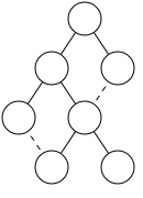
figure 7
Threads are a method for reducing the amount of time it takes to scan a subtree for its contour by creating links between nodes on the contour if one is not already the child of the other. In Figure 7, the dotted line represents a thread while a solid line represents a parent-child relationship.
We can also take advantage of the fact that, if the one tree is deeper than the other, we only need to descend as far as the shorter tree. Anything deeper than that will not affect the separation necessary between the two trees, since there can be no conflicts between them.
Using threads and only traversing as deeply as we need to, we can get a contour for a tree and set our threads in linear time with the procedure in Listing 8.
def nextright(tree):
    if tree.thread:   return tree.thread
    if tree.children: return tree.children[-1]
    else:             return None

def nextleft(tree):
    if tree.thread:   return tree.thread
    if tree.children: return tree.children[0]
    else:             return None

def contour(left, right, max_offset=0, left_outer=None, right_outer=None):
    if not left_outer:
        left_outer = left
    if not right_outer:
        right_outer = right

    if left.x - right.x > max_offset:
        max_offset = left.x - right.x

    lo = nextleft(left)
    li = nextright(left)
    ri = nextleft(right)
    ro = nextright(right)

    if li and ri:
        return contour(li, ri, max_offset, lo, ro)

    return max_offset
It's easy to see that this procedure only visits two nodes on each level of the subtree being scanned. The paper has a neat proof that this occurs in linear time; I recommend that you go read it if you're interested.
Putting it all Together
The contour procedure given in Listing 8 is neat and fast, but it won't work with the mod technique we discussed earlier, because the actual x value of a node is the node's x value plus the sum of all the modifiers on the path from itself to the root. To handle this case, we'll need to add another couple bits of complexity to our contour algorithm.
The first thing we need to do is maintain two additional variables, a sum of the modifiers on the left subtree and a sum of the modifiers on the right subtree. These sums are necessary to compute the actual position of each node on the contour, so that we can check to see if it conflicts with a node on the opposite side. See Listing 9.
def contour(left, right, max_offset=None, loffset=0, roffset=0, left_outer=None, right_outer=None):
    delta = left.x + loffset - (right.x + roffset)
    if not max_offset or delta > max_offset:
        max_offset = delta

    if not left_outer:
        left_outer = left
    if not right_outer:
        right_outer = right

    lo = nextleft(left_outer)
    li = nextright(left)
    ri = nextleft(right)
    ro = nextright(right_outer)

    if li and ri:
        loffset += left.mod
        roffset += right.mod
        return contour(li, ri, max_offset,
                       loffset, roffset, lo, ro)

    return (li, ri, max_offset, loffset, roffset, left_outer, right_outer)
The other thing we need to do is return the current state of the function when we exit so that we can set the proper offset on the threaded nodes. With that information in hand, we're ready to look at the function that uses the code in Listing 8 to place two trees as closely together as possible:
def fix_subtrees(left, right):
    li, ri, diff, loffset, roffset, lo, ro \
        = contour(left, right)
    diff += 1
    diff += (right.x + diff + left.x) % 2

    right.mod = diff
    right.x += diff

    if right.children:
        roffset += diff

    if ri and not li:
        lo.thread = ri
        lo.mod = roffset - loffset
    elif li and not ri:
        ro.thread = li
        ro.mod = loffset - roffset

    return (left.x + right.x) / 2
After we run the contour procedure, we add 1 to the maximum difference between the left and right trees so that they won't conflict with each other, then add another one if the midpoint between them is odd. This lets us keep a handy property for testing - all nodes have integral x coordinates, with no loss of precision.
Then we move the right tree the prescribed amount to the right. Remember here that the reason we both add diff to the x coordinate and save it to the mod value is that the mod value only applies to the nodes below the current node. If the right subtree has more than one node, we add diff to the roffset, since all children of the right node will be moved that far to the right.
If the left side of the tree was deeper than the right, or vice versa, we need to set a thread. We simply check to see if the node pointer for one side progressed farther than the node pointer for the other side, and if it has, set the thread from the outside of the shallower tree to the inside of the deeper one.
In order to properly handle the mod values that we talked about before, we need to set a special mod value on threaded nodes. Since we've already updated our right offset value to reflect the right tree's movement to the right, all we need to do here is set the mod value of the threaded node to the difference between the offset of the deeper tree and itself.
Now that we have code in place to find the contours of trees and to place two trees as close together as possible, we can easily implement the algorithm described above. I present the rest of the code without comment:
def layout(tree):
    return addmods(setup(dt))

def addmods(tree, mod=0):
    tree.x += mod
    for c in tree.children:
        addmods(c, mod+tree.mod)
    return tree

def setup(tree, depth=0):
    if len(tree.children) == 0:
        tree.x = 0
        tree.y = depth
        return tree

    if len(tree.children) == 1:
        tree.x = setup(tree.children[0], depth+1).x
        return tree

    left = setup(tree.children[0], depth+1)
    right = setup(tree.children[1], depth+1)

    tree.x = fix_subtrees(left, right)
    return tree
Extension to N-ary Trees
Now that we've finally got an algorithm for drawing binary trees which satisfies our principles, looks good in the general case, and runs in linear time, it's natural to think about how to extend it to trees with any amount of children. If you've followed me this far, you're probably thinking that we should just take the wonderful algorithm we've just defined and apply it across all the children of a node.
An extension of the previous algorithm to work on n-ary trees might look something like this:
- Do a post-order traversal of the tree
- if the node is a leaf, give it an x coordinate of 0
- otherwise, for each of its children, place the child as close to its left sibling as possible
- place the parent node halfway between its leftmost and rightmost children
Principle 6: The child nodes of a parent node should be evenly spaced.
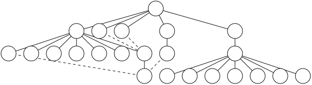
figure 8
In order to draw an n-ary tree symmetrically, and quickly, we're going to need all the tricks we've developed so far plus a couple of new ones. Thanks to a recent paper by Christoph Buchheim et al5, we've got all the tools at hand to do so and still be able to draw our trees in linear time.
To modify the algorithm above to meet Principle 6, we'll need a method for spacing out the trees in between two larger trees that conflict. The simplest method would be to, every time two trees conflict, divide the available space by the number of trees, and shift each tree so that it's separated by that amount from its siblings. For example, in Figure 8, there is some distance n between the large trees on the right and the left, and three trees in between them. If we simply spaced the first tree in the middle n/3 away from the left tree, the next one n/3 away from that, and so on, we'd have a tree that satisfied Principle 6.
Every time so far that we've looked at a simple algorithm in this article, we've found it inadequate, and this time is no different. If we have to shift all the trees in between every two trees that conflict, we run the risk of introducing an O(n^2) operation into our algorithm.
The fix for this problem is similar to the fix for the previous shifting problem we had, for which we introduced mod. Instead of shifting each subtree in the middle every time we have a conflict, we'll save the value that we need to shift the trees in the middle, then apply the shifts after we've placed all the children of a node.
In order to figure out the correct value we want to shift the middle nodes, we'll need to be able to find the number of trees in between the two nodes that conflict. When we only had two trees, it was obvious that any conflict that occurred was between the left and the right tree. When there may be any number of trees, finding out which tree is causing the conflict becomes a challenge.
To meet this challenge, we'll introduce a default_ancestor variable and add another member to our tree data structure, which we'll call the ancestor. The ancestor node either points to itself or to the root of the tree it belongs to. When we need to find which tree a node belongs to, we'll use the ancestor member if it is set, but fall back on the tree pointed to by default_ancestor.
When we place the first subtree of a node, we simply set default_ancestor to point to that subtree, and assume that any conflict caused by the next tree is with the first one. After we've placed the second subtree, we distinguish two cases. If the second subtree is less deep than the first, we traverse its right contour, setting the ancestor member equal to the root of the second tree. Otherwise, the second tree is larger than the first, which means that any conflicts with the next tree to be placed with be with the second tree, and so we simply set default_ancestor to point to it.
So, without further ado, a python implementation of the O(n) algorithm for laying out attractive trees as presented by Buchheim is in Listing 12.
class DrawTree(object):
    def __init__(self, tree, parent=None, depth=0, number=1):
        self.x = -1.
        self.y = depth
        self.tree = tree
        self.children = [DrawTree(c, self, depth+1, i+1)
                         for i, c
                         in enumerate(tree.children)]
        self.parent = parent
        self.thread = None
        self.offset = 0
        self.ancestor = self
        self.change = self.shift = 0
        self._lmost_sibling = None
        #this is the number of the node in its group of siblings 1..n
        self.number = number

    def left_brother(self):
        n = None
        if self.parent:
            for node in self.parent.children:
                if node == self: return n
                else:            n = node
        return n

    def get_lmost_sibling(self):
        if not self._lmost_sibling and self.parent and self != \
        self.parent.children[0]:
            self._lmost_sibling = self.parent.children[0]
        return self._lmost_sibling
    leftmost_sibling = property(get_lmost_sibling)

def buchheim(tree):
    dt = firstwalk(tree)
    min = second_walk(dt)
    if min < 0:
        third_walk(dt, -min)
    return dt

def firstwalk(v, distance=1.):
    if len(v.children) == 0:
        if v.leftmost_sibling:
            v.x = v.left_brother().x + distance
        else:
            v.x = 0.
    else:
        default_ancestor = v.children[0]
        for w in v.children:
            firstwalk(w)
            default_ancestor = apportion(w, default_ancestor,
                                         distance)
        execute_shifts(v)

        midpoint = (v.children[0].x + v.children[-1].x) / 2

        ell = v.children[0]
        arr = v.children[-1]
        w = v.left_brother()
        if w:
            v.x = w.x + distance
            v.mod = v.x - midpoint
        else:
            v.x = midpoint
    return v

def apportion(v, default_ancestor, distance):
    w = v.left_brother()
    if w is not None:
        #in buchheim notation:
        #i == inner; o == outer; r == right; l == left;
        vir = vor = v
        vil = w
        vol = v.leftmost_sibling
        sir = sor = v.mod
        sil = vil.mod
        sol = vol.mod
        while vil.right() and vir.left():
            vil = vil.right()
            vir = vir.left()
            vol = vol.left()
            vor = vor.right()
            vor.ancestor = v
            shift = (vil.x + sil) - (vir.x + sir) + distance
            if shift > 0:
                a = ancestor(vil, v, default_ancestor)
                move_subtree(a, v, shift)
                sir = sir + shift
                sor = sor + shift
            sil += vil.mod
            sir += vir.mod
            sol += vol.mod
            sor += vor.mod
        if vil.right() and not vor.right():
            vor.thread = vil.right()
            vor.mod += sil - sor
        else:
            if vir.left() and not vol.left():
                vol.thread = vir.left()
                vol.mod += sir - sol
            default_ancestor = v
    return default_ancestor

def move_subtree(wl, wr, shift):
    subtrees = wr.number - wl.number
    wr.change -= shift / subtrees
    wr.shift += shift
    wl.change += shift / subtrees
    wr.x += shift
    wr.mod += shift

def execute_shifts(v):
    shift = change = 0
    for w in v.children[::-1]:
        w.x += shift
        w.mod += shift
        change += w.change
        shift += w.shift + change

def ancestor(vil, v, default_ancestor):
    if vil.ancestor in v.parent.children:
        return vil.ancestor
    else:
        return default_ancestor

def second_walk(v, m=0, depth=0, min=None):
    v.x += m
    v.y = depth

    if min is None or v.x < min:
        min = v.x

    for w in v.children:
        min = second_walk(w, m + v.mod, depth+1, min)

    return min

def third_walk(tree, n):
    tree.x += n
    for c in tree.children:
        third_walk(c, n)
Conclusion
I've glossed over a few things in this article, simply because I felt it was more important to try and present a logical progression to the final algorithm I presented than it was to overload the article with pure code. If you want more details, or to see the tree data structures that I've used in the various code listings, you can go to http://github.com/llimllib/pymag-trees/ to download the source code for each algorithm, some basic tests, and the code used to generate the figures for this article.
Footnotes
1 K. Marriott, NP-Completeness of Minimal Width Unordered Tree Layout, Journal of Graph Algorithms and Applications, vol. 8, no. 3, pp. 295-312 (2004). http://www.emis.de/journals/JGAA/accepted/2004/MarriottStuckey2004.8.3.pdf
2 D. E. Knuth, Optimum binary search trees, Acta Informatica 1 (1971)
3 C. Wetherell, A. Shannon, Tidy Drawings of Trees, IEEE Transactions on Software Engineering. Volume 5, Issue 5
4 E. M. Reingold, J. S Tilford, Tidier Drawings of Trees, IEEE Transactions on Software Engineering. Volume 7, Issue 2
5 C. Buchheim, M. J Unger, and S. Leipert. Improving Walker's algorithm to run in linear time. In Proc. Graph Drawing (GD), 2002. http://citeseerx.ist.psu.edu/viewdoc/download?doi=10.1.1.16.8757